How phase transfer entropy works

One pair of oscillators, X driving Y, followed from raw phase to a connectivity graph. Every number and figure on this page is computed when the documentation is built; the drawing code lives in examples/utils/teaching.py.

\[\mathrm{PTE}(X \to Y) = H(Y_{t+\delta} \mid Y_t) - H(Y_{t+\delta} \mid Y_t, X_t)\]

In words: how much less uncertain Y’s next phase becomes once you also know X’s current phase. The steps below build each piece of that line.

The example pair

Two delayed Kuramoto oscillators where X drives Y, and nothing flows back. Steps 1 to 3 use a long run so the histograms are smooth; steps 4 and 5 use recordings of realistic length. Phase is cut into 12 equal bins throughout, so the probabilities drawn are exactly the ones pyPTE counts.

import warnings

import numpy as np

from examples.models import kuramoto
from examples.utils import style, teaching
from pyPTE import PTE, surrogate_test
from pyPTE.core.pyPTE import get_delay, get_phase

style.use()
K = 12
PAIR = dict(noise=1.0, freq_spread=0.5)
DRIVE = np.array([[0, 4.0], [0, 0]])

signal = kuramoto.simulate(DRIVE, n_samples=300_000, seed=2, **PAIR)
phase = get_phase(signal)
delay = get_delay(phase)
codes = np.clip(np.floor((phase + np.pi) / (2 * np.pi / K)), 0, K - 1).astype(int)
dPTE, raw_PTE = PTE(signal, binning=K, delay=delay)

x, y = codes
y_now, y_future = y[:-delay], y[delay:]
x_now, x_future = x[:-delay], x[delay:]
print(
    f"delay {delay} samples, PTE X→Y {raw_PTE[0, 1]:.3f} bits, "
    f"Y→X {raw_PTE[1, 0]:.3f} bits, dPTE {dPTE[0, 1]:.2f}"
)

/home/runner/work/pyPTE/pyPTE/pyPTE/core/pyPTE.py:481: RuntimeWarning: 12 phase bins: with fewer than 16, the direction dPTE reports for a real coupling can depend on the delay, even flipping sign; significance against chance is unaffected. To rely on the direction, set binning to 16 or more.
  d_phase, analysis_delay, n_bins = prepare_phase(
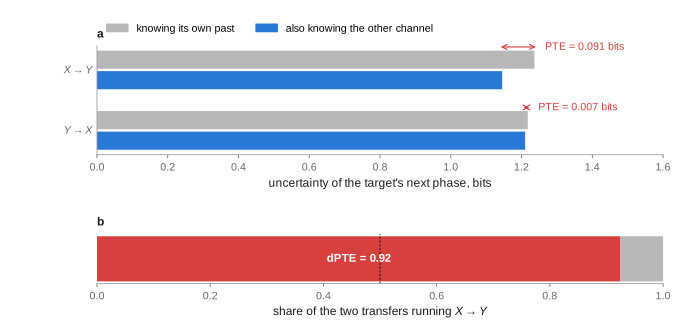
delay 12 samples, PTE X→Y 0.091 bits, Y→X 0.007 bits, dPTE 0.92

1. Entropy measures how spread out a phase is

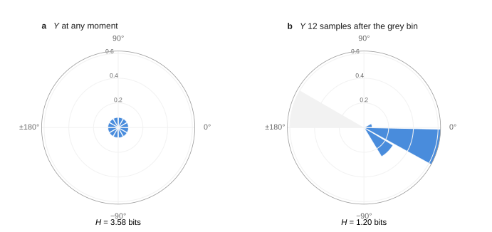
Entropy \(H\) is the average number of yes/no questions needed to pin down which bin a value falls in: largest for a flat histogram, zero for a single spike. Conditional entropy \(H(A \mid B)\) is the same once \(B\) is known.

Over the whole recording Y visits every bin equally (a). But 12 samples after Y sat in one bin, it has almost always moved half a cycle on (b): knowing where Y was cuts its uncertainty sharply.

held = int(np.bincount(y_now).argmax())
anywhere = np.bincount(y, minlength=K) / y.size
after = np.bincount(y_future[y_now == held], minlength=K)
after = after / after.sum()

teaching.rose_pair(anywhere, after, held, delay)

2. Transfer means X sharpens Y’s future even further

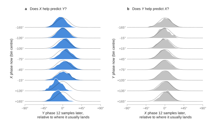
Hold Y’s current bin fixed and split its future by X’s current phase. Each ridge in a is Y’s future for one bin of X; the dashed outline ignores X. The peaks move away from the outline, so each is narrower: X carries information about where Y goes. In b the roles are swapped and every ridge sits on its outline. Bins of the other channel that hardly occur alongside the held bin are left out.

Transfer entropy is that drop in conditional entropy, the conditional mutual information \(I(Y_{t+\delta} ; X_t \mid Y_t)\). Phase transfer entropy computes it on Hilbert phases, so amplitude plays no part.

teaching.ridgelines(phase, codes, delay, held)

3. One number per direction, and their ratio

A conditional entropy is the entropy of the joint state minus the entropy of what is given. pyPTE packs each joint state into one integer, one base-12 digit per variable, and counts those integers; the same trick works here.

Each pair of bars in a is one direction: the uncertainty of the target’s future given its own past, then given the other channel as well. The gap is PTE. dPTE in b is X→Y’s share of the two transfers, \(\mathrm{PTE}(X\to Y) / (\mathrm{PTE}(X\to Y) + \mathrm{PTE}(Y\to X))\). It answers “which way?”, not “how strong?”, and 0.5 means no net direction.

def encode(*variables):
    state = np.zeros_like(variables[0])
    for v in variables:
        state = state * K + v
    return state


def conditional_entropy(future, *given):
    joint = teaching.entropy(np.bincount(encode(future, *given)))
    return joint - teaching.entropy(np.bincount(encode(*given)))


rows = [
    (
        r"$X \rightarrow Y$",
        conditional_entropy(y_future, y_now),
        conditional_entropy(y_future, y_now, x_now),
    ),
    (
        r"$Y \rightarrow X$",
        conditional_entropy(x_future, x_now),
        conditional_entropy(x_future, x_now, y_now),
    ),
]
teaching.entropy_bars(rows)

4. A value is only meaningful against its own null

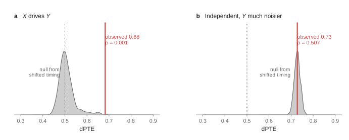
A surrogate test rebuilds the statistic many times on data where the effect cannot exist, here by shifting each channel’s timing at random, which keeps each signal intact but breaks their alignment. The p-value is the share of surrogates at least as extreme as the real value.

The coupled pair lands far outside its null (a). Two independent signals with Y much noisier land even further from 0.5, but so does their whole null (b): the cleaner channel is easier to predict and looks like a driver. dPTE alone cannot tell these apart; the null can.

rng = np.random.default_rng(4)
coupled = kuramoto.simulate(DRIVE, n_samples=12_000, seed=3, **PAIR)
coupled += 0.2 * rng.standard_normal(coupled.shape)
unrelated = kuramoto.simulate(np.zeros((2, 2)), n_samples=12_000, seed=5, **PAIR)
unrelated += np.array([[0.2], [1.5]]) * rng.standard_normal(unrelated.shape)

results = [
    surrogate_test(data, n_surrogates=1000, seed=0, keep_null=True, binning=K)
    for data in (coupled, unrelated)
]
teaching.null_densities(results, ["$X$ drives $Y$", "Independent, $Y$ much noisier"])

/home/runner/work/pyPTE/pyPTE/pyPTE/stats.py:572: RuntimeWarning: 12 phase bins: with fewer than 16, the direction dPTE reports for a real coupling can depend on the delay, even flipping sign; significance against chance is unaffected. To rely on the direction, set binning to 16 or more.
  d_phase, analysis_delay, n_bins = prepare_phase(

5. Many short recordings beat one long one

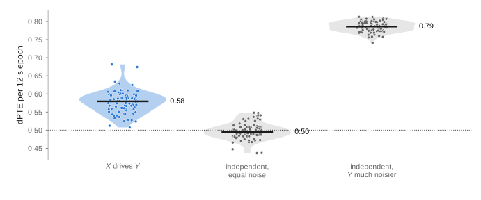
Each dot is one 12 s epoch. Coupled epochs sit above 0.5 almost every time, a consistency that pyPTE.group_test() detects easily. The noisy-Y condition sits higher still with no coupling at all, which is why conditions are compared with each other rather than with 0.5.

def epoch_dpte(coupling, noise_y, seed):
    data = kuramoto.simulate(coupling, n_samples=3000, seed=seed, **PAIR)
    noise = np.array([[0.2], [noise_y]])
    data += noise * np.random.default_rng(seed).standard_normal(data.shape)
    return PTE(data, binning=K)[0][0, 1]


independent = np.zeros((2, 2))
groups = {
    "$X$ drives $Y$": np.array([epoch_dpte(DRIVE, 0.2, 100 + s) for s in range(80)]),
    "independent,\nequal noise": np.array(
        [epoch_dpte(independent, 0.2, 300 + s) for s in range(80)]
    ),
    "independent,\n$Y$ much noisier": np.array(
        [epoch_dpte(independent, 1.5, 300 + s) for s in range(80)]
    ),
}
fig, ax = teaching.violins(groups, highlight="$X$ drives $Y$")
ax.set_ylabel("dPTE per 12 s epoch")

/home/runner/work/pyPTE/pyPTE/pyPTE/core/pyPTE.py:481: RuntimeWarning: 12 phase bins: with fewer than 16, the direction dPTE reports for a real coupling can depend on the delay, even flipping sign; significance against chance is unaffected. To rely on the direction, set binning to 16 or more.
  d_phase, analysis_delay, n_bins = prepare_phase(

6. Significant edges make a graph, with predictable errors

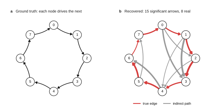
Eight oscillators in a ring, each driving the next (a). Only edges surviving the surrogate test with false-discovery-rate control are drawn in b, width by dPTE − 0.5. Direction is right on every arrow, but some arrows skip a node: information really does flow that way, through an intermediate, and a pairwise measure cannot tell a direct connection from an indirect one.

The false discovery rate bounds the expected share of false edges among those reported. With 28 channel pairs, pyPTE.surrogates_needed() says how many surrogates an isolated edge needs before it can pass at all.

ring_coupling = kuramoto.ring_with_shortcut(8, strength=3.0)
ring = kuramoto.simulate(ring_coupling, n_samples=12_000, seed=1)
with warnings.catch_warnings():
    warnings.simplefilter("ignore")
    ring_result = surrogate_test(ring, n_surrogates=1200, seed=0)

teaching.network_pair(kuramoto.net_flow(ring_coupling), ring_result)

7. At brain scale, flow is not anatomy

The same lesson grows with the network. On a 76-region connectome almost every pair of regions is joined by a short indirect route, and the strongest dPTE flows rarely coincide with direct anatomical tracts; see Flow vs anatomy at brain scale.